OptimalTransportNetworks.jl

Optimal Transport Networks in Spatial Equilibrium - in Julia

Modern Julia (JuMP) translation of the MATLAB OptimalTransportNetworkToolbox (v1.0.4b) implementing the quantitative spatial economic model of:

Fajgelbaum, P. D., & Schaal, E. (2020). Optimal transport networks in spatial equilibrium. Econometrica, 88(4), 1411-1452.

The model/software uses duality principles to optimize over the space of networks, nesting an optimal flows problem and a neoclasical general-equilibrium trade model into a global network design problem to derive the optimal (welfare maximizing) transport network (extension) from any primitive set of economic fundamantals [population per location, productivity per location for each of N traded goods, endowment of a non-traded good, and (optionally) a pre-existing transport network].

For more information about the model see this folder and the MATLAB User Guide. See also my blog post on this software release.

The model is the first of its kind and a pathbreaking contribution towards the welfare maximizing planning of transport infrastructure. Its creation has been funded by the European Union through an ERC Research Grant. The author of this Julia library has no personal connections to the authors, but has used their Matlab library for research purposes and belives that it deserves an accessible open-source implementation. Community efforts to further improve the code are welcome.

Example

The code for this example is in example04.jl. See the examples folder for more examples.

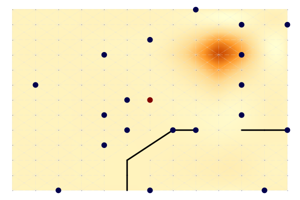
This plot shows the endowments on a map-graph: circle size is population, circle colour is productivity (the central node is more productive), the black lines indicate geographic barriers, and the background is shaded according to the cost of network building (elevation), indicating a mountain in the upper right corner.

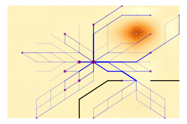
This plot shows the optimal network after 200 iterations, keeping population fixed and not allowing for cross-good congestion. The size of nodes indicates consumption in each node.

Performance Notes

As of v0.3.0, the default solver path calls Ipopt directly (via its C interface) with hard-coded sparse gradients, Jacobians, and Hessians — like the original MATLAB toolbox — for all Armington cases (at most one good produced per location), across fixed / partial / full labor mobility, with or without cross-good congestion. The Ipopt problem is built once and reused (warm-started) across the network-design iterations. This is several times to an order of magnitude faster than the JuMP path at realistic graph sizes, and the gap widens as the graph grows. The fixed-labor, beta <= 1 case additionally uses the even-faster dual solution (duality = true by default).
JuMP (and its automatic differentiation) is now an opt-in fallback: set jump = true in init_parameters to force it. The general, non-Armington case (a location producing two or more goods) is not covered by the hand-coded solvers and always uses JuMP, regardless of the jump switch.
Symbolic autodifferentiation via MathOptSymbolicAD.jl can also provide significant performance improvements for non-dual cases. The symbolic backend can be activated using:

import MathOptInterface as MOI
import MathOptSymbolicAD

param[:model_attr] = Dict(:backend => (MOI.AutomaticDifferentiationBackend(), 
                                       MathOptSymbolicAD.DefaultBackend())) 
                                # Or:  MathOptSymbolicAD.ThreadedBackend()

It is recommended to use Coin-HSL linear solvers for Ipopt to speed up computations. In my opinion the simplest way to use them is to get a (free for academics) license and download the binaries here, extract them somewhere, and then set the hsllib (place here the path to where you extracted libhsl.dylib, it may also be called libcoinhsl.dylib, in which case you may have to rename it to libhsl.dylib) and linear_solver options as follows:

param[:optimizer_attr] = Dict(:hsllib => "/usr/local/lib/libhsl.dylib", # Adjust path
                              :linear_solver => "ma57") # Use ma57, ma86 or ma97

The Ipopt.jl README suggests to use the larger LibHSL package for which there exists a Julia module and proceed similarly. In addition, users may try an optimized BLAS and see if it yields significant performance gains (and let me know if it does).